決定木 (分類)(DecisionTreeClassifier) のしくみと実装解説

本記事では、XGBoostをはじめとするGBDTモデルの基礎にある、決定木(分類) (Decision Tree Classifier) の仕組みについて、初学者にもわかりやすいように実装コードとともに説明していきます。

---

決定木とは？

決定木は、データを特徴に基づいて「木構造」で分類するアルゴリズムです。

• 特徴:
  • 各ノード（節点）で、ある特徴量とその閾値による二分割を行う
  • 葉ノード（終端ノード）では、最も多く出現するクラスラベルを予測値として採用する

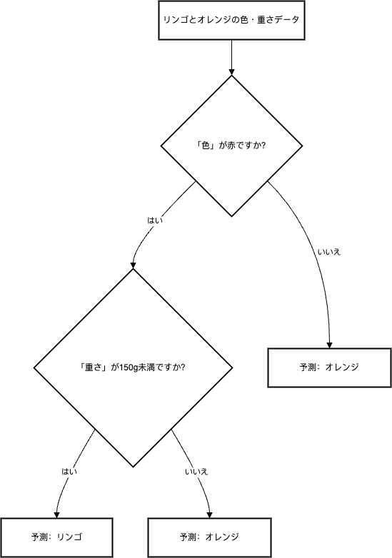
たとえば、「ある果物がリンゴかオレンジか」 を分類する場合、

• 「色」や「重さ」などの特徴により木を分岐し、最終的に「リンゴ」または「オレンジ」を予測する、といったイメージです。

---

数式で見る決定木の基本概念

Gini不純度

決定木の各ノードで、データの「純度」を評価するために Gini不純度 が用いられます。
Gini不純度は、あるノード内でランダムに選んだサンプルが誤分類される確率を示します。

値が小さいほど、そのノードは誤分類が少なく「純粋」であるといえます。

Gini 不純度の数式:

$$ \text{Gini} = 1 – \sum_{c=1}^{C} \left(\frac{n_c}{m}\right)^2 $$

• \( m \): ノード内のサンプル数
• \( n_c \): クラス \( c \) のサンプル数
• \( C \): クラスの総数

情報利得

情報利得は、ある分割によって Gini不純度 がどれだけ減少するかを表す指標です。
分割前の不純度から、左右の子ノードの不純度の重み付き平均を引いた値が情報利得となります。

Information Gain の数式:

$$ \text{Information Gain} = Gini_{parent} – \left(\frac{n_{left}}{n} \times Gini_{left} + \frac{n_{right}}{n} \times Gini_{right}\right) $$

• \( n \): 親ノードのサンプル数
• \( n_{left} \) と \( n_{right} \): 左右の子ノードのサンプル数

分割の候補の中で情報利得が最大になるものを選び、最適な分割とします。

---

実装の流れ

決定木の実装は、概ね以下の流れで進みます。

1. ノードの定義
   各ノードを表現するクラスを作成します。ここでは、分割に用いる特徴量のインデックスや閾値、左右の子ノード、または葉ノードの予測値を保持します。
2. 再帰的な木の成長
   トップノードから始め、条件（最大深度、サンプル数、同一クラスなど）を満たすまで、再帰的にノードを分割していきます。
   各ノードで最適な特徴量と閾値の組み合わせを探索し、左右に分けます。
3. 予測処理
   新しいサンプルに対して、ルートから始めて各ノードの条件を順に確認し、最終的にたどり着いた葉ノードの予測値を返します。

---

部分的な実装コード

以下は、上記の各要素に対応するコードの一部です。

Node クラス

from collections import Counter

# Node class
class Node:
    def __init__(self, feature_index=None, threshold=None, left=None, right=None, *, value=None):
        # Index of feature used for split
        self.feature_index = feature_index  
        # Threshold value for split
        self.threshold = threshold          
        # Left child node
        self.left = left                    
        # Right child node
        self.right = right                  
        # Predicted class for leaf node (if not None, node is a leaf)
        self.value = value                  

    def is_leaf_node(self):
        return self.value is not None

DecisionTreeClassifier クラス（主要部分）

import numpy as np

# Custom Decision Tree Classifier implementation
class DecisionTreeClassifier:
    def __init__(self, min_samples_split=2, max_depth=100, n_features=None):
        # Minimum number of samples required to split a node
        self.min_samples_split = min_samples_split  
        # Maximum depth of the tree
        self.max_depth = max_depth                  
        # Number of features to consider when looking for the best split (if None, use all)
        self.n_features = n_features                
        self.root = None

    # Fit the model on the training data
    def fit(self, X, y):
        self.n_classes_ = len(set(y))
        self.n_features_ = X.shape[1]
        if self.n_features is None:
            self.n_features = self.n_features_
        self.root = self._grow_tree(X, y)

    # Recursively build the tree
    def _grow_tree(self, X, y, depth=0):
        n_samples, n_features = X.shape
        n_labels = len(np.unique(y))

        # Stop criteria: max depth reached, all samples have the same label, or not enough samples to split
        if (depth >= self.max_depth or n_labels == 1 or n_samples < self.min_samples_split):
            leaf_value = self._most_common_label(y)
            return Node(value=leaf_value)

        # Randomly select features (if n_features is less than total number of features)
        feature_idxs = np.random.choice(n_features, self.n_features, replace=False)

        # Find the best split among the selected features
        best_feat, best_thresh = self._best_split(X, y, feature_idxs)
        if best_feat is None:
            leaf_value = self._most_common_label(y)
            return Node(value=leaf_value)

        # Split the data based on the best feature and threshold
        left_idxs = X[:, best_feat] <= best_thresh
        right_idxs = X[:, best_feat] > best_thresh

        # Recursively build left and right subtrees
        left = self._grow_tree(X[left_idxs], y[left_idxs], depth + 1)
        right = self._grow_tree(X[right_idxs], y[right_idxs], depth + 1)
        return Node(feature_index=best_feat, threshold=best_thresh, left=left, right=right)

    # Determine the best split by calculating information gain using Gini impurity
    def _best_split(self, X, y, feature_idxs):
        best_gain = -1
        split_idx, split_thresh = None, None

        for feat_idx in feature_idxs:
            X_column = X[:, feat_idx]
            thresholds = np.unique(X_column)
            for threshold in thresholds:
                gain = self._information_gain(y, X_column, threshold)
                if gain > best_gain:
                    best_gain = gain
                    split_idx = feat_idx
                    split_thresh = threshold

        return split_idx, split_thresh

    # Calculate information gain using the decrease in Gini impurity
    def _information_gain(self, y, X_column, split_thresh):
        parent_gini = self._gini(y)

        left_idxs = X_column <= split_thresh
        right_idxs = X_column > split_thresh

        # If either split is empty, no information gain is achieved
        if len(y[left_idxs]) == 0 or len(y[right_idxs]) == 0:
            return 0

        n = len(y)
        n_left, n_right = len(y[left_idxs]), len(y[right_idxs])
        gini_left, gini_right = self._gini(y[left_idxs]), self._gini(y[right_idxs])
        weighted_gini = (n_left / n) * gini_left + (n_right / n) * gini_right

        gain = parent_gini - weighted_gini
        return gain

    # Compute the Gini impurity for a set of labels
    def _gini(self, y):
        m = len(y)
        return 1.0 - sum((np.sum(y == c) / m) ** 2 for c in np.unique(y))

    # Return the most common label in the set
    def _most_common_label(self, y):
        from collections import Counter
        counter = Counter(y)
        most_common = counter.most_common(1)[0][0]
        return most_common

    # Predict the class for each sample in X
    def predict(self, X):
        return np.array([self._traverse_tree(x, self.root) for x in X])

    # Recursively traverse the tree to make a prediction
    def _traverse_tree(self, x, node):
        if node.is_leaf_node():
            return node.value
        if x[node.feature_index] <= node.threshold:
            return self._traverse_tree(x, node.left)
        return self._traverse_tree(x, node.right)

---

完成版のコード

以下は、上記の各部分を統合した、完成版のカスタム DecisionTreeClassifier のコードです。
また、軽量なデータセット（ここでは Iris データセット）を用いて、実際に学習・予測を行う例も含めています。

import numpy as np
import pandas as pd
from collections import Counter
from sklearn.datasets import load_iris
from sklearn.model_selection import StratifiedKFold
from sklearn.metrics import accuracy_score
from tqdm import tqdm

# ---------------------------
# Node class representing a tree node
# ---------------------------
class Node:
    def __init__(self, feature_index=None, threshold=None, left=None, right=None, *, value=None):
        # Index of feature used for split
        self.feature_index = feature_index  
        # Threshold value for split
        self.threshold = threshold          
        # Left child node
        self.left = left                    
        # Right child node
        self.right = right                  
        # Predicted class for leaf node (if not None, node is a leaf)
        self.value = value                  

    def is_leaf_node(self):
        return self.value is not None

# ---------------------------
# Custom Decision Tree Classifier implementation
# ---------------------------
class DecisionTreeClassifier:
    def __init__(self, min_samples_split=2, max_depth=100, n_features=None):
        # Minimum number of samples required to split a node
        self.min_samples_split = min_samples_split  
        # Maximum depth of the tree
        self.max_depth = max_depth                  
        # Number of features to consider when looking for the best split (if None, use all)
        self.n_features = n_features                
        self.root = None

    # Fit the model on the training data
    def fit(self, X, y):
        self.n_classes_ = len(set(y))
        self.n_features_ = X.shape[1]
        if self.n_features is None:
            self.n_features = self.n_features_
        self.root = self._grow_tree(X, y)

    # Recursively build the tree
    def _grow_tree(self, X, y, depth=0):
        n_samples, n_features = X.shape
        n_labels = len(np.unique(y))

        # Stop criteria: max depth reached, all samples have the same label, or not enough samples to split
        if (depth >= self.max_depth or n_labels == 1 or n_samples < self.min_samples_split):
            leaf_value = self._most_common_label(y)
            return Node(value=leaf_value)

        # Randomly select features (if n_features is less than total number of features)
        feature_idxs = np.random.choice(n_features, self.n_features, replace=False)

        # Find the best split among the selected features
        best_feat, best_thresh = self._best_split(X, y, feature_idxs)
        if best_feat is None:
            leaf_value = self._most_common_label(y)
            return Node(value=leaf_value)

        # Split the data based on the best feature and threshold
        left_idxs = X[:, best_feat] <= best_thresh
        right_idxs = X[:, best_feat] > best_thresh

        # Recursively build left and right subtrees
        left = self._grow_tree(X[left_idxs], y[left_idxs], depth + 1)
        right = self._grow_tree(X[right_idxs], y[right_idxs], depth + 1)
        return Node(feature_index=best_feat, threshold=best_thresh, left=left, right=right)

    # Determine the best split by calculating information gain using Gini impurity
    def _best_split(self, X, y, feature_idxs):
        best_gain = -1
        split_idx, split_thresh = None, None

        for feat_idx in feature_idxs:
            X_column = X[:, feat_idx]
            thresholds = np.unique(X_column)
            for threshold in thresholds:
                gain = self._information_gain(y, X_column, threshold)
                if gain > best_gain:
                    best_gain = gain
                    split_idx = feat_idx
                    split_thresh = threshold

        return split_idx, split_thresh

    # Calculate information gain using the decrease in Gini impurity
    def _information_gain(self, y, X_column, split_thresh):
        parent_gini = self._gini(y)

        left_idxs = X_column <= split_thresh
        right_idxs = X_column > split_thresh

        # If either split is empty, no information gain is achieved
        if len(y[left_idxs]) == 0 or len(y[right_idxs]) == 0:
            return 0

        n = len(y)
        n_left, n_right = len(y[left_idxs]), len(y[right_idxs])
        gini_left, gini_right = self._gini(y[left_idxs]), self._gini(y[right_idxs])
        weighted_gini = (n_left / n) * gini_left + (n_right / n) * gini_right

        gain = parent_gini - weighted_gini
        return gain

    # Compute the Gini impurity for a set of labels
    def _gini(self, y):
        m = len(y)
        return 1.0 - sum((np.sum(y == c) / m) ** 2 for c in np.unique(y))

    # Return the most common label in the set
    def _most_common_label(self, y):
        counter = Counter(y)
        most_common = counter.most_common(1)[0][0]
        return most_common

    # Predict the class for each sample in X
    def predict(self, X):
        return np.array([self._traverse_tree(x, self.root) for x in X])

    # Recursively traverse the tree to make a prediction
    def _traverse_tree(self, x, node):
        if node.is_leaf_node():
            return node.value
        if x[node.feature_index] <= node.threshold:
            return self._traverse_tree(x, node.left)
        return self._traverse_tree(x, node.right)

# ---------------------------
# Demonstration with the Iris dataset
# ---------------------------
if __name__ == '__main__':
    # Load the Iris dataset
    iris = load_iris()
    X = iris.data
    y = iris.target

    # Use Stratified K-Fold cross-validation for demonstration
    folds = 5
    skf = StratifiedKFold(n_splits=folds, shuffle=True, random_state=42)
    oof_preds = np.zeros(len(X))
    test_preds = np.zeros(len(X))  # For demonstration, we use the same data as test

    # Cross-validation loop with a progress bar
    for fold, (train_idx, val_idx) in enumerate(tqdm(list(skf.split(X, y)), total=folds, desc="Folds")):
        print(f"\nFold {fold+1}/{folds}")
        
        X_train, y_train = X[train_idx], y[train_idx]
        X_val, y_val = X[val_idx], y[val_idx]

        # Create and train the custom Decision Tree Classifier
        model = DecisionTreeClassifier(max_depth=5, min_samples_split=2)
        model.fit(X_train, y_train)
        
        # Predict on the validation set
        val_preds = model.predict(X_val)
        oof_preds[val_idx] = val_preds
        
        acc = accuracy_score(y_val, val_preds)
        print(f"Fold {fold+1} Accuracy: {acc:.4f}")
        
        # For demonstration, assign validation predictions as test predictions
        test_preds[val_idx] = model.predict(X_val)

    overall_acc = accuracy_score(y, oof_preds)
    print(f"\nOverall Accuracy: {overall_acc:.4f}")
    print("Test Predictions:", test_preds)

---

まとめ

本記事では、決定木(分類)の基本概念、数学的背景、そして実装の流れを詳しく解説しました。
もし本記事の内容に誤りや改善点があれば、コメントいただければ幸いです。

付録: 回帰の場合

回帰木における分割基準（分散の減少）の数式:

$$ \text{Reduction} = \text{Var}_{parent} – \left(\frac{n_{left}}{n} \times \text{Var}_{left} + \frac{n_{right}}{n} \times \text{Var}_{right}\right) $$

• \( n \): 親ノードのサンプル数
• \( n_{left} \) と \( n_{right} \): 左右の子ノードのサンプル数
• \( \text{Var}_{parent} \), \( \text{Var}_{left} \), \( \text{Var}_{right} \): それぞれ親ノード、左ノード、右ノードの分散

分類木との違い:
分類木では、各ノードの純度を評価するためにGini不純度やエントロピーを用い、情報利得（不純度の減少）を基準として分割を行います。一方、回帰木では、目的変数の分散（または平均二乗誤差）の減少量を評価基準とし、分割前後の分散の差（分散の減少）が最大になるような分割を選びます。